Convert RGB three band to single band colour table

This function converts a three-band SpatialGridDataFrame into a single band of colour indices and a colour look-up table using RGB2PCT. vec2RGB uses given breaks and colours (like image) to make a three column matrix of red, green, and blue values for a numeric vector.

SGDF2PCT(x, ncolors = 256, adjust.bands=TRUE)
vec2RGB(vec, breaks, col)

Arguments

x

a three-band SpatialGridDataFrame object

ncolors

a number of colours between 2 and 256

adjust.bands

default TRUE; if FALSE the three bands must lie each between 0 and 255, but will not be streched within those bounds

vec

a numeric vector

breaks

a set of breakpoints for the colours: must give one more breakpoint than colour

col

a list of colors

Value

The value returned is a list:

idx

a vector of colour indices in the same spatial order as the input object

ct

a vector of RGB colours

References

https://gdal.org/

Author

Roger Bivand

Examples

logo <- system.file("pictures/Rlogo.jpg", package="rgdal")[1]
SGlogo <- readGDAL(logo)
#> Warning: GDAL support is provided by the sf and terra packages among others
#> /tmp/RtmpnkEu0w/temp_libpath101e75200293a/rgdal/pictures/Rlogo.jpg has GDAL driver JPEG 
#> and has 175 rows and 200 columns
#> Warning: GDAL support is provided by the sf and terra packages among others
#> Warning: GeoTransform values not available
cols <- SGDF2PCT(SGlogo)
SGlogo$idx <- cols$idx
image(SGlogo, "idx", col=cols$ct)

SGlogo <- readGDAL(logo)
#> Warning: GDAL support is provided by the sf and terra packages among others
#> /tmp/RtmpnkEu0w/temp_libpath101e75200293a/rgdal/pictures/Rlogo.jpg has GDAL driver JPEG 
#> and has 175 rows and 200 columns
#> Warning: GDAL support is provided by the sf and terra packages among others
#> Warning: GeoTransform values not available
cols <- SGDF2PCT(SGlogo, ncolors=64)
SGlogo$idx <- cols$idx
image(SGlogo, "idx", col=cols$ct)

SGlogo <- readGDAL(logo)
#> Warning: GDAL support is provided by the sf and terra packages among others
#> /tmp/RtmpnkEu0w/temp_libpath101e75200293a/rgdal/pictures/Rlogo.jpg has GDAL driver JPEG 
#> and has 175 rows and 200 columns
#> Warning: GDAL support is provided by the sf and terra packages among others
#> Warning: GeoTransform values not available
cols <- SGDF2PCT(SGlogo, ncolors=8)
SGlogo$idx <- cols$idx
image(SGlogo, "idx", col=cols$ct)

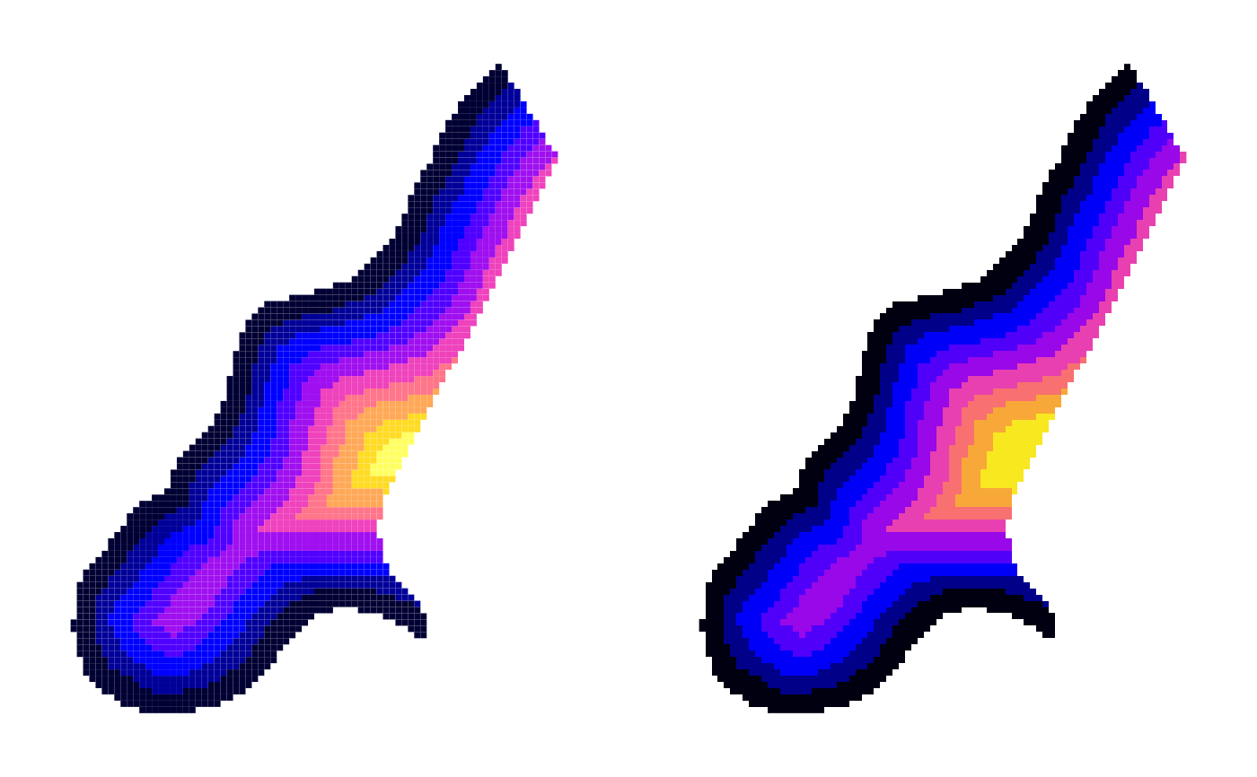
data(meuse.grid)
coordinates(meuse.grid) <- c("x", "y")
gridded(meuse.grid) <- TRUE
fullgrid(meuse.grid) <- TRUE
summary(meuse.grid$dist)
#>    Min. 1st Qu.  Median    Mean 3rd Qu.    Max.    NA's 
#>   0.000   0.119   0.272   0.297   0.440   0.993    5009 
opar <- par(no.readonly=TRUE)
par(mfrow=c(1,2), mar=c(1,1,1,1)+0.1)
image(meuse.grid, "dist", breaks=seq(0,1,1/10), col=bpy.colors(10))
RGB <- vec2RGB(meuse.grid$dist, breaks=seq(0,1,1/10), col=bpy.colors(10))
summary(RGB)
#>       red             green             blue      
#>  Min.   :  0.00   Min.   :  0.00   Min.   : 36.0  
#>  1st Qu.:  0.00   1st Qu.:  0.00   1st Qu.: 87.0  
#>  Median :  0.00   Median :  0.00   Median :189.0  
#>  Mean   : 75.31   Mean   : 22.98   Mean   :171.1  
#>  3rd Qu.:159.00   3rd Qu.: 15.00   3rd Qu.:255.0  
#>  Max.   :255.00   Max.   :255.00   Max.   :255.0  
#>  NA's   :5009     NA's   :5009     NA's   :5009   
meuse.grid$red <- RGB[,1]
meuse.grid$green <- RGB[,2]
meuse.grid$blue <- RGB[,3]
cols <- SGDF2PCT(meuse.grid[c("red", "green", "blue")], ncolors=10,
 adjust.bands=FALSE)
is.na(cols$idx) <- is.na(meuse.grid$dist)
meuse.grid$idx <- cols$idx
image(meuse.grid, "idx", col=cols$ct)

par(opar)
# Note: only one wrongly classified pixel after NA handling/dropping
# The functions are not written to be reversible
sort(table(findInterval(meuse.grid$dist, seq(0,1,1/10), all.inside=TRUE)))
#> 
#>  10   9   8   7   6   5   4   2   3   1 
#>  28  54  99 118 237 417 431 507 525 687 
sort(table(cols$idx))
#> 
#>  10   1   2   3   4   6   5   9   7 
#>  82  99 118 237 417 431 507 525 687